

Stoyan R. Vezenkov
Center for applied neuroscience Vezenkov, BG-1582 Sofia, e-mail: info@vezenkov.com
For citation: Vezenkov, S.R. (2025) From Prime Rays to a Paired 12×5 Slot Torus with Applications to Discrete Sequence Encodings. Nootism 1(6), 44-52, https://doi.org/10.64441/nootism.1.6.4
Abstract
We introduce a modular-ray representation of integers by mapping each n ∈ ℤ to the polar ray determined by its residue modulo 360. For primes p > 5, admissible directions are exactly the 96 reduced residues in (ℤ/360ℤ)×, which split canonically along the unconditional 6k ± 1 scaffold into two arithmetic threads of 48 rays each (A: 6k − 1, B: 6k + 1).
On top of this arithmetic layer we define a paired 12×5 slot container—one 12×5 table per thread—aligned with the natural 12-sector decomposition modulo 30. Within each thread, the 48 admissible rays are placed into four slots across the 12 sectors (12×4 = 48), while the fifth slot is reserved for explicitly designated composite-ray channels that appear as controlled leakage states in the discrete transition rules. We then embed the resulting 60-slot container via a dodecahedral incidence model (12 faces × 5 per-face incidences), yielding a purely combinatorial adjacency suitable for defining discrete dynamics and operator constraints. Throughout, we keep the unconditional scaffold and explicit Ray-ID tables distinct from optional interpretation and application layers.
As an application, we show how the same 60/96 container can be instantiated as a discrete encoding layer for DNA by combining strand, phase bins, and a base alphabet with an explicit reverse-complement involution. This yields a compact, symmetry-aware tokenization and graph structure that can be used as inductive bias in deep learning models for sequence classification and time-resolved genomics.
Keywords: prime numbers; modular rays; Ray-ID alphabet; residues mod 360; 6k±1 threads; paired 12×5 slot torus; 12-sector decomposition; composite-ray channels; zero-bridge involution; dodecahedral incidence graph; 96→60 refinement; DNA sequence encoding.
1. Introduction and scope
Prime numbers satisfy rigid modular constraints while exhibiting irregular global distribution. A standard arithmetic scaffold is the decomposition into the two progressions 6k±1, which contain all primes larger than 3. (Vezenkov, 2025) The Euler product representation of ζ(s) serves as the analytic prototype for our ray grouping, emphasizing the multiplicative independence of prime factors that we preserve in the geometric model. (Edwards, 1974)
This paper develops a precise structural framework that (i) represents candidate prime locations as modular rays (congruence classes), (ii) enumerates admissible prime rays by ray IDs, and (iii) organizes these ray addresses into a 12×5 slot lattice whose adjacency is supplied by a dodecahedral incidence container.
1.1. Layering
To avoid conflating unconditional arithmetic statements with model-specific structure, we separate the paper into layers. L0 (unconditional arithmetic scaffold): the two progressions 6k±1 contain all primes p>3. L1 (structural state space): two threads (A/B), a sign (+/−), and a 12×5 slot lattice equipped with a dodecahedral incidence identification and adjacency. L2 (instantiation data): explicit slot-encoding tables Φ_A, Φ_B that assign ray IDs (directed residue classes) to slot addresses. L3 (derived operators and testable constraints): adjacency/transition operators induced by the dodecahedral incidence and the zero-bridge J acting as a deterministic state transition on slot addresses. L4 (optional application layer): the same two-strand + phase/slot container can be reused as a representation layer for other two-strand sequences (e.g., DNA) and for equivariant deep-learning; this does not add number-theoretic claims and is clearly marked as optional.
2. Structural core: threads, sign, and the slot container
2.1. Two candidate threads on the positive branch
Define A⁺(k) := 6k−1 and B⁺(k) := 6k+1 for k ∈ N. These two threads contain all primes p>3, but composite values occur abundantly on both. As established by Dirichlet's theorem on arithmetic progressions, the linear forms 6k±1 contain infinitely many primes, forming the asymptotic density foundation upon which our two threads rest.(Davenport, 2013)
2.2. Crossed negative branch and the zero-bridge concept
A naive extension to negative integers reflects n ↦ −n. We instead use crossed reflection so that a sign change induces a thread swap with respect to the k-indexing: A⁻(k) := −B⁺(k)=−(6k+1) and B⁻(k) := −A⁺(k)=−(6k−1). This realizes +5=A⁺(1) ↦ −7=A⁻(1) and +7=B⁺(1) ↦ −5=B⁻(1).
2.3. Bridge operator J as an involution on the scaffold
Let a⁺(k):=6k−1 and b⁺(k):=6k+1 for k∈ℕ, and define the associated thread sets A⁺:={a⁺(k):k∈ℕ}, B⁺:={b⁺(k):k∈ℕ}. Define the crossed negative branch by a⁻(k):=−b⁺(k)=−(6k+1) and b⁻(k):=−a⁺(k)=−(6k−1), with A⁻:={a⁻(k)} and B⁻:={b⁻(k)}. Let H:=A⁺∪B⁺∪A⁻∪B⁻. The zero-bridge operator is the involution J:H→H given by J(a⁺(k))=a⁻(k), J(b⁺(k))=b⁻(k), and conversely J(a⁻(k))=a⁺(k), J(b⁻(k))=b⁺(k). Equivalently, for n∈A⁺ (i.e., n≡−1 (mod 6), n>0) one has J(n)=−(n+2), and for n∈B⁺ (n≡+1 (mod 6), n>0) one has J(n)=−(n−2); the negative-branch rules are the inverse maps. Note that J preserves the formal thread label c∈{A,B} on the signed scaffold. The apparent A↔B swap is an effective one when a negative-branch value is re-expressed as a positive-branch progression (since A⁻=−B⁺ and B⁻=−A⁺).
2.4. Slot space and dodecahedral incidence (defined jointly)
We define a 60-slot structural container in two complementary ways: (i) as a coordinate torus for indexing and (ii) as a dodecahedral incidence structure that supplies adjacency relations.
(i) Coordinate torus (indexing). Let F=Z₁₂ and V=Z₅. Define S := F×V, so |S|=12·5=60. We refer to f∈F as a face index and v∈V as a slot index within the face.
(ii) Dodecahedral incidence container (combinatorial geometry). Let D be a regular dodecahedron. For each face g∈Faces(D), let Vert(g) denote its five vertices. Define the incidence set I := {(g,u): g∈Faces(D), u∈Vert(g)}, so |I|=12·5=60. A dodecahedral labeling is a bijection Ψ:I→S. Once Ψ is fixed, any explicitly stated incidence rule (e.g., edge-sharing, vertex-sharing) induces an adjacency relation on S.
(iii) Signed double-thread state space. Introduce a thread label c∈{A,B} and a sign label s∈{+,-}. The resulting state space is S_double := {A,B}×{+,-}×S (240 discrete address states) prior to any radial indexing.
3. Modular rays modulo 360 and the 12-sector decomposition
3.1. Ray map modulo 360
Fix M:=360. For n∈ℤ define r(n):=n mod M and θ(n):=2π·r(n)/M. A ray ℛ_a is the congruence class {n∈ℤ : n≡a (mod M)}. Plotting integers by polar coordinates (ρ(n),θ(n)) for any monotone radius ρ produces straight rays indexed by residues a. The orthogonality properties of Dirichlet characters provide the classical basis for partitioning residues, a structure we here geometrize explicitly via the ray projection.(Apostol, 2013)
Figures 1–3 visualize this ray geometry for primes on the A and B threads.
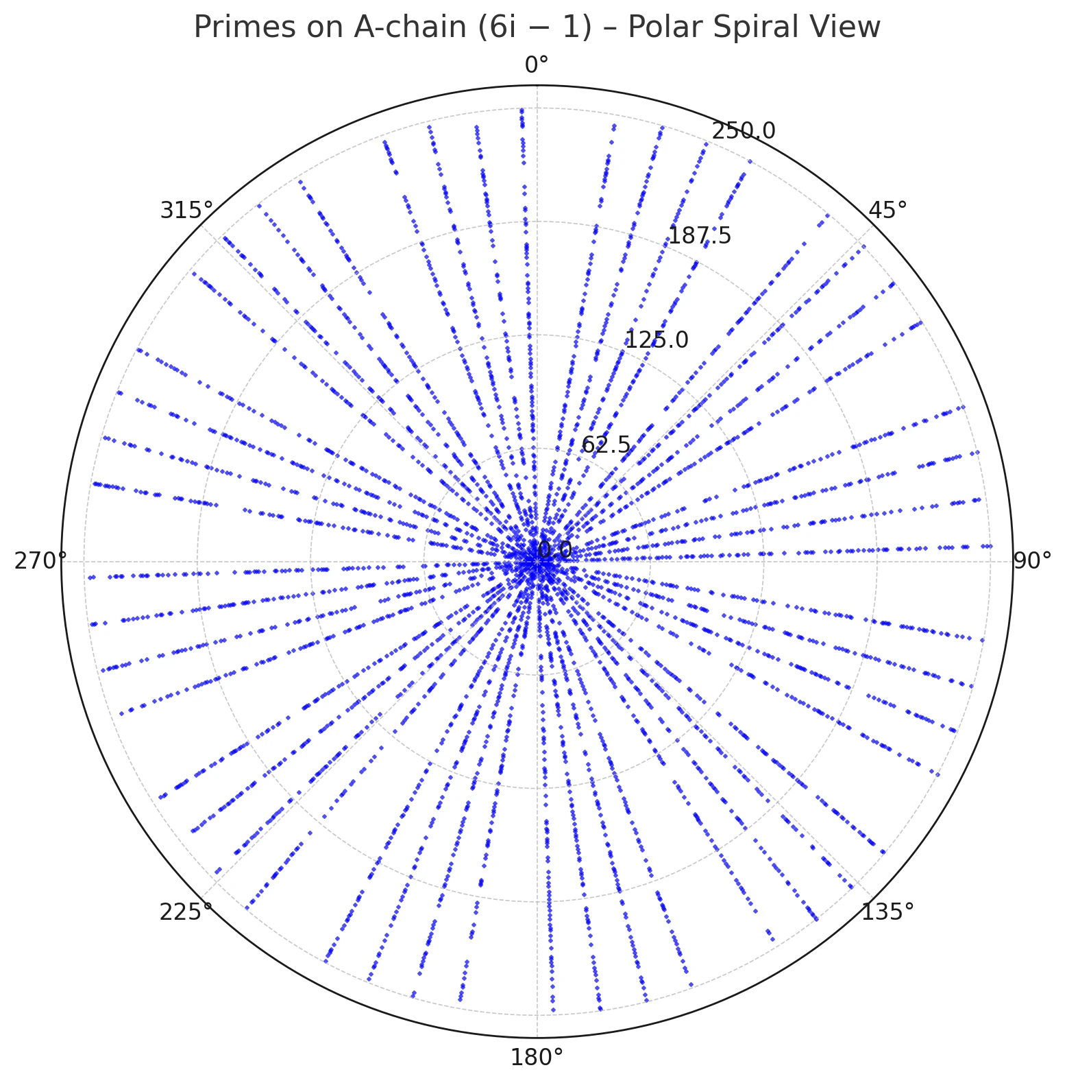
Figure 1. Primes on the A-chain (6k−1) plotted in polar coordinates by residue modulo 360; points align on admissible rays.
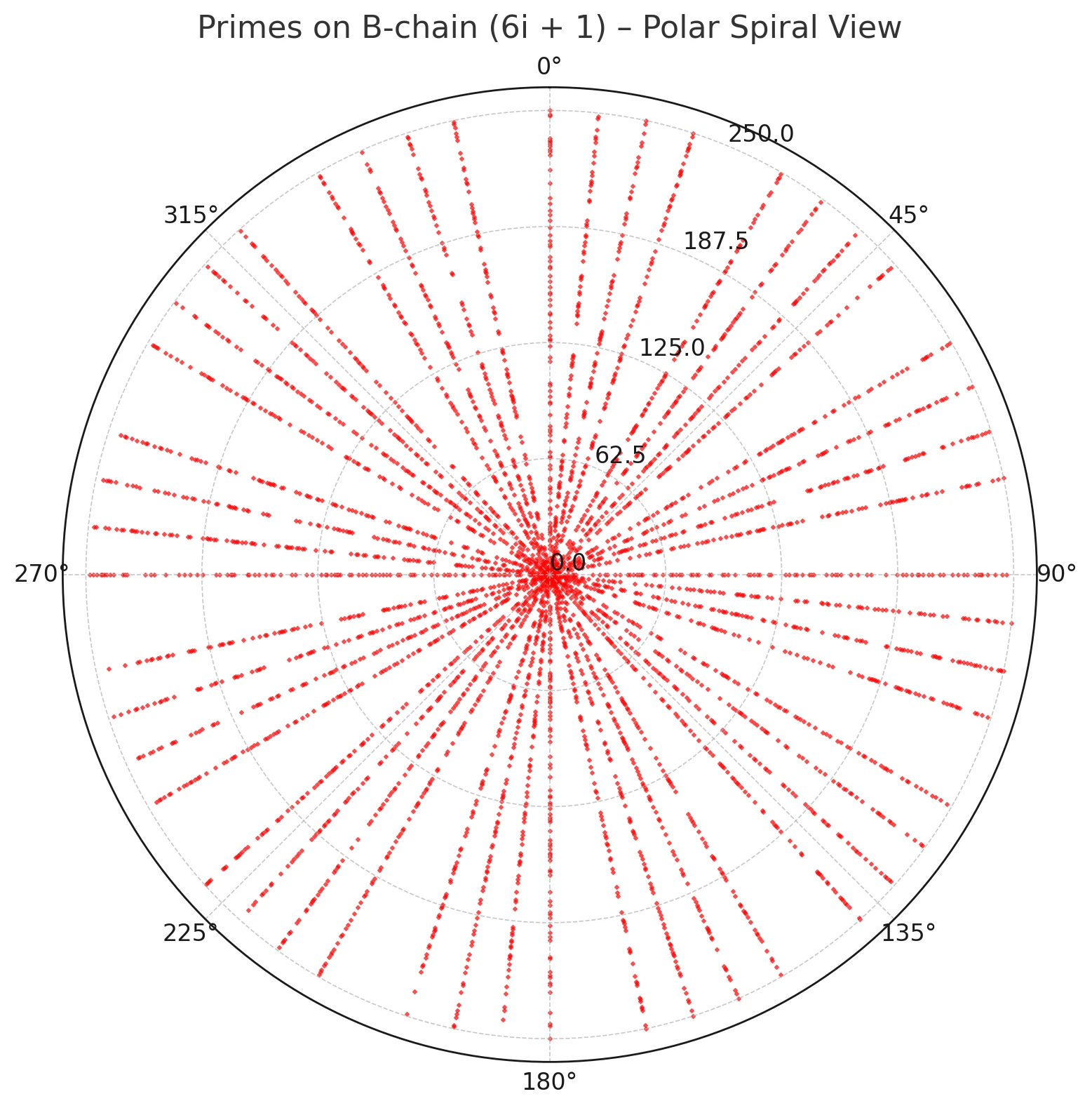
Figure 2. Primes on the B-chain (6k+1) plotted in polar coordinates by residue modulo 360; points align on admissible rays.
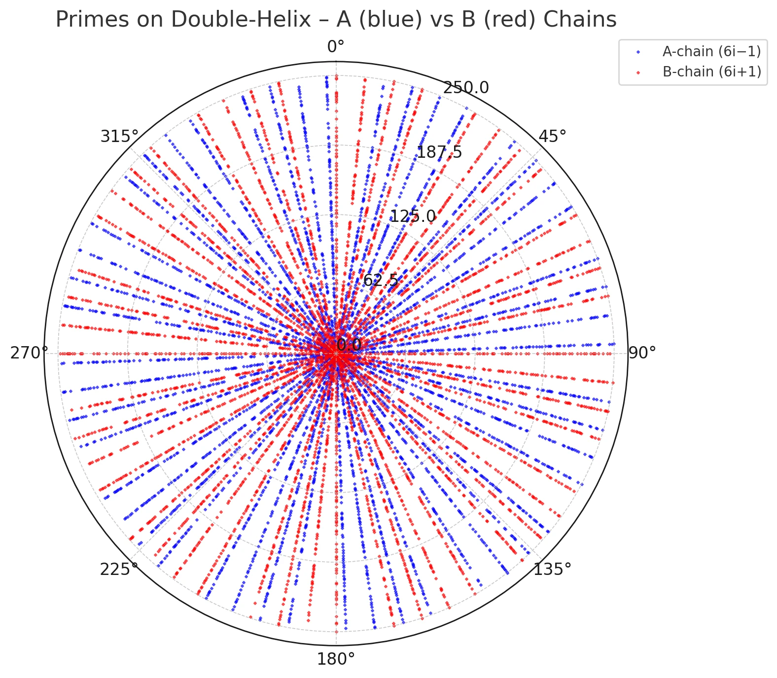
Figure 3. Overlay of A (blue) and B (red) prime rays; the two families interleave in angular direction.
3.2. Admissible rays for primes p>5 and the ray-ID alphabet
Let := {a∈{0,…,359} : gcd(a,360)=1}. Then |𝒰| = φ(360)=96. For any prime p>5, the residue r(p)=p mod 360 lies in 𝒰. Note that elements of 𝒰 need not be prime as integers; they are units modulo 360 and only encode admissible ray directions.
Table 3.1. Ray IDs for admissible residues modulo 360 (Instantiation I: increasing-residue order).
| 1 | 2 | 3 | 4 | 5 | 6 | 7 | 8 |
| 1:1 | 2:7 | 3:11 | 4:13 | 5:17 | 6:19 | 7:23 | 8:29 |
| 9:31 | 10:37 | 11:41 | 12:43 | 13:47 | 14:49 | 15:53 | 16:59 |
| 17:61 | 18:67 | 19:71 | 20:73 | 21:77 | 22:79 | 23:83 | 24:89 |
| 25:91 | 26:97 | 27:101 | 28:103 | 29:107 | 30:109 | 31:113 | 32:119 |
| 33:121 | 34:127 | 35:131 | 36:133 | 37:137 | 38:139 | 39:143 | 40:149 |
| 41:151 | 42:157 | 43:161 | 44:163 | 45:167 | 46:169 | 47:173 | 48:179 |
| 49:181 | 50:187 | 51:191 | 52:193 | 53:197 | 54:199 | 55:203 | 56:209 |
| 57:211 | 58:217 | 59:221 | 60:223 | 61:227 | 62:229 | 63:233 | 64:239 |
| 65:241 | 66:247 | 67:251 | 68:253 | 69:257 | 70:259 | 71:263 | 72:269 |
| 73:271 | 74:277 | 75:281 | 76:283 | 77:287 | 78:289 | 79:293 | 80:299 |
| 81:301 | 82:307 | 83:311 | 84:313 | 85:317 | 86:319 | 87:323 | 88:329 |
| 89:331 | 90:337 | 91:341 | 92:343 | 93:347 | 94:349 | 95:353 | 96:359 |
3.3. The 12-sector (mod 30) decomposition and why “12×5” is natural
We partition residues modulo 360 into 12 sectors of width 30: sector f corresponds to residues {30f,30f+1,…,30f+29}. Within each sector, the admissible residues are exactly the eight unit classes modulo 30.
Specifically, the unit classes modulo 30 are {1,7,11,13,17,19,23,29}. Proof sketch: a residue class is admissible iff it is coprime to 2·3·5=30; the units modulo 30 are precisely those eight classes because φ(30)=8.
4. Slot encoding Φ_A, Φ_B (explicit 12×5 tables)
We now fix a concrete instantiation of the slot encoding maps Φ_A, Φ_B. Crucially, the tables are not arbitrary: face index f is identified with the mod-30 sector B_f, and the four prime-ray slots per face are exactly the four admissible offsets for that thread within the sector.
4.1. Address alphabet and slot order
Let the ray-ID alphabet be := {1,…,96} as in Table 3.1. We extend it by two composite markers to obtain the extended ray alphabet 𝓡_ext := {1,…,96} ∪ {C5, C25}. The markers C5 and C25 correspond to the composite offsets 5 and 25, i.e., residues 30f+5 and 30f+25 within a sector f.
4.2. Explicit tables
Define Φ_B(f,v)=id(30f+offset_B[v]) for v=0..3 and Φ_B(f,4)=C5; define Φ_A(f,v)=id(30f+offset_A[v]) for v=0..3 and Φ_A(f,4)=C25, where offset_B=[1,7,13,19] and offset_A=[11,17,23,29]. Tables 4.1–4.2 list the resulting IDs.
Table 4.1. Φ_A (A-thread slot table; face f = sector 30f..30f+29).
| face f | v0 | v1 | v2 | v3 | v4 |
| 0 | 3 | 5 | 7 | 8 | C25 |
| 1 | 11 | 13 | 15 | 16 | C25 |
| 2 | 19 | 21 | 23 | 24 | C25 |
| 3 | 27 | 29 | 31 | 32 | C25 |
| 4 | 35 | 37 | 39 | 40 | C25 |
| 5 | 43 | 45 | 47 | 48 | C25 |
| 6 | 51 | 53 | 55 | 56 | C25 |
| 7 | 59 | 61 | 63 | 64 | C25 |
| 8 | 67 | 69 | 71 | 72 | C25 |
| 9 | 75 | 77 | 79 | 80 | C25 |
| 10 | 83 | 85 | 87 | 88 | C25 |
| 11 | 91 | 93 | 95 | 96 | C25 |
Table 4.2. Φ_B (B-thread slot table; face f = sector 30f..30f+29).
| face f | v0 | v1 | v2 | v3 | v4 |
| 0 | 1 | 2 | 4 | 6 | C5 |
| 1 | 9 | 10 | 12 | 14 | C5 |
| 2 | 17 | 18 | 20 | 22 | C5 |
| 3 | 25 | 26 | 28 | 30 | C5 |
| 4 | 33 | 34 | 36 | 38 | C5 |
| 5 | 41 | 42 | 44 | 46 | C5 |
| 6 | 49 | 50 | 52 | 54 | C5 |
| 7 | 57 | 58 | 60 | 62 | C5 |
| 8 | 65 | 66 | 68 | 70 | C5 |
| 9 | 73 | 74 | 76 | 78 | C5 |
| 10 | 81 | 82 | 84 | 86 | C5 |
| 11 | 89 | 90 | 92 | 94 | C5 |
5. Dodecahedral incidence embedding Ψ and induced adjacency
Let 𝒟 be a regular dodecahedron. The combinatorial incidence properties of the regular dodecahedron, particularly the face-vertex connectivity, provide the rigid adjacency skeleton necessary to define discrete dynamics without topological ambiguity. (Coxeter, 1973) Let Faces(𝒟) be its 12 faces and Vert(f) be the 5 vertices of a face f. The incidence set is I := {(f,v) : f∈Faces(𝒟), v∈Vert(f)}, so |I|=12·5=60. A slot embedding is any bijection Ψ:I→S, which identifies the 12×5 container with dodecahedral face–vertex incidences.
We define Ψ:I→S by Ψ(face=g, position=i)=(f=g, v=i). With this choice, S is simultaneously (i) a coordinate index set and (ii) a labeled dodecahedral incidence set. Any alternative labeling corresponds to permuting face indices and/or cyclically shifting the v index within faces.
5.1. Adjacency operators on S
We use two explicit adjacency generators derived from the dodecahedron:
We define two operators on the incidence container S := 𝕫₁₂×𝕫₅.
• Within-face rotation R: R(f,v) := (f, v+1 mod 5).
- Edge transfer E: for each state (f,v), consider the oriented edge from vertex v to v+1 on face f. Let f′ be the unique neighboring face sharing this edge and let v′ be the index on f′ of the same starting vertex. Define E(f,v) := (f′,v′). Appendix A.2 lists E(f,v) for all (f,v)∈S.
- Induced adjacency: the undirected adjacency on S is generated by {R, R⁻¹, E, E⁻¹}. For a directed graph one may use only {R, E}.
These operators generate a nontrivial adjacency graph on S (and therefore on S_double once thread and sign labels are added).
6. The zero-bridge as a state transition on slot addresses (A↔B flip and composite leakage)
On the arithmetic scaffold H, J implements crossed reflection: J(6k−1)=−(6k+1) and J(6k+1)=−(6k−1). This section translates J into a deterministic transition on signed slot states.
6.1. Signed slot states
A signed slot state is a tuple (c,s,f,v) ∈ {A,B}×{+,-}×Z₁₂×Z₅. On the positive branch (s=+), the pair (c,f,v) addresses a ray direction via Tables 4.1–4.2 (with v=4 denoting a composite channel). The bridge J maps s=+ states to s=− states and implements crossed reflection on the 6k±1 scaffold (A⁺→A⁻=−B⁺, B⁺→B⁻=−A⁺), which appears as an interchange between A-type and B-type admissible offsets at the ray level.
6.2. Local transition rules in the mod-30 sector model
Because J differs from simple sign reflection by a ±2 shift, its action is most transparent in the mod-30 sector representation. Within a sector f, the B offsets are [1,7,13,19] and the A offsets are [11,17,23,29]. Adding/subtracting 2 stays within the same sector except at the boundary offsets 29 and 1, which wrap to the next/previous sector. Moreover, exactly one offset per thread hits a multiple of 5: 7−2=5 and 23+2=25. This yields controlled transitions into the composite channels C5 and C25.
Proposition 6.1 (bridge transition on positive-slot addresses).
We list the induced transitions on (c,s,f,v), separating them by the originating thread. Composite leakage into v4 is treated as thread-preserving by convention; alternatively, composite markers may be treated as thread-neutral.
• Transitions originating from B (positive branch):
(B,+,f,v1) ↦ (A,−,f,v1) [offset 1 ↦ offset 29],
(B,+,f,v2) ↦ (A,−,f,v2) [offset 11 ↦ offset 19],
(B,+,f,v3) ↦ (A,−,f,v3) [offset 13 ↦ offset 17],
(B,+,f,v4) ↦ (B,−,f,v4) [offset 7 ↦ composite offset 5 = C5].
• Transitions originating from A (positive branch):
(A,+,f,v1) ↦ (B,−,f,v1) [offset 29 ↦ offset 1],
(A,+,f,v2) ↦ (B,−,f,v2) [offset 19 ↦ offset 11],
(A,+,f,v3) ↦ (B,−,f,v3) [offset 17 ↦ offset 13],
(A,+,f,v4) ↦ (A,−,f,v4) [offset 23 ↦ composite offset 25 = C25].
This explicit transition captures the intended “5↔7 flip” across zero at the scaffold level (A⁺ maps to A⁻=−B⁺ and B⁺ maps to B⁻=−A⁺) while remaining compatible with the modular-ray picture: almost all rays map between admissible rays, with a small, structured leakage into C5/C25.
7. Genomic representation layer: a DNA instantiation and modern genetics tasks (optional)
This section is independent of the prime-ray instantiation. It treats the double-strand (two-channel) structure and the 12-phase slot container as a generic discrete representation layer. The intent is methodological: to encode biologically standard objects (diploid genomes and DNA sequences) in a way that makes strand symmetry and helical phase explicit for machine learning. No biological mechanism is claimed.
7.1. Diploid genome addressing (2×23 chromosomes)
Let Hap := {0,1} index haplotypes in a diploid setting (hap1/hap2). For sex chromosomes and aneuploid contexts Hap may be partially defined; we treat Hap as a generic ploidy index. Let Chr := {1,…,22,X,Y} denote chromosomes, and for each chromosome c let Pos(c):={0,…,L(c)−1}. A genomic coordinate is (h,c,i) with h∈Hap, c∈Chr, i∈Pos(c), together with an optional orientation o∈{+,-}.
7.2. Two-strand tokenization with 12 phase bins and reverse-complement operators
To incorporate helical periodicity as a regularizing feature, we attach a phase-bin index p(i)∈𝕫₁₂ to each position i. For B-DNA this should be interpreted as discrete binning of a continuous helical phase (not as a claim of 12 bp per turn). One concrete choice is p(i)=⌊12·frac(i/10.5)⌋, where frac(x)=x−⌊x⌋.
Let Σ:={A,C,G,T} be the nucleotide alphabet and let Str:={W,C} denote the two strands (Watson/Crick). These strand labels are independent of the prime threads A/B used elsewhere in the model. Define the DNA token space X_DNA := 𝕫₁₂ × Str × Σ. For position i and strand σ∈Str we represent the nucleotide as x(i,σ):=(p(i),σ,b(i,σ)). Complementarity is the involution comp on Σ given by comp(A)=T, comp(T)=A, comp(C)=G, comp(G)=C, combined with a strand swap W↔C: Comp(p,W,b)=(p,C,comp(b)) and Comp(p,C,b)=(p,W,comp(b)). Reverse-complement equivariance on a length-n window is the composition of Comp with index reversal i↦(n−1−i).
Optional 12×5 embedding: if we wish to reuse the 12×5 slot lattice, we can map the four bases to four slots v∈{0,1,2,3} on each face and reserve v=4 as a meta-channel. The meta-channel can encode biologically meaningful annotations such as CpG methylation (5mC), ambiguity/quality (“N”), local conformation class (B/A/Z), or chromatin state; this makes the fifth slot a data-bearing channel rather than a placeholder.
7.3. Why the representation can help deep learning and priority genetics problems
The value of the encoding is not compression (raw DNA is already optimally encodable), but inductive bias: (i) explicit reverse-complement symmetry; (ii) an explicit helical phase channel; and (iii) a fixed small token alphabet (96 states) that can be used in transformer/GNN pipelines without hand-crafted k-mers. While modern models like DNABERT use k-mer tokenization to extract context, our approach offers an alternative structural bias based on fixed phase constraints and strand symmetry.(Ji et al., 2021)
Three immediately testable use-cases are:
1) Non-coding variant effect prediction and regulatory annotation. Models predicting enhancer/promoter activity, TF binding, or chromatin features from sequence should be invariant/equivariant to reverse complement. Encoding RC symmetry as a fixed operator can reduce sample complexity and improve generalization.
2) Structural variants (SV), repeats, and difficult regions. SV breakpoints are context-dependent and often lie in repetitive sequence. Local windows can be represented as walks in X_DNA, and SV contexts can be summarized by slot/ray statistics; these features can be attached to graph models of rearrangements.
3) Pangenome / graph reference representations. As the field moves toward graph-based references, node/edge attributes can be defined by distributions over X_DNA (and optionally 12×5 meta-channels), enabling learned embeddings of pangenome segments and ancestry-aware comparisons.
A minimal publication-quality evaluation is to train a baseline sequence model (one-hot or k-mer tokenization) and a model using the X_DNA encoding with explicit reverse-complement equivariance on a standard benchmark (e.g., enhancer classification or variant effect). Performance and data-efficiency differences are directly measurable, making this layer falsifiable.
7.4. Scope and claim (what is and is not claimed)
We introduce an application layer that represents time-resolved single-cell gene expression as an event log indexed by (i) canonical biological identifiers and (ii) the 60/96 structural container. The representation is lossless with respect to recorded observations (event log + checkpoints), not with respect to the underlying biological trajectory (which is typically not directly observed in single-cell snapshot datasets).
7.5. Three-layer specification (Address → Structural token → Expression events)
7.5.1. Layer 1: biological address (canonical, lossless identifier)
Let g ∈ G be a gene (or transcript). Define a canonical biological address
a(g) := (gene_id, chr, start, end, strand),
where gene_id is a stable reference ID and strand ∈ {+,-} is the genomic strand.
Let c ∈ C be a cell. The minimal cell identity is a(c) := (cell_id), optionally extended by a measurement context record
m(c) := (batch_id, library_size, qc_flags, platform).
7.5.2. Layer 2: structural tokenization on the 60/96 container
The principal value of the container is not compression of raw sequences, but the ability to inject structure (strand/reverse-complement symmetry, phase regularization, and an explicit adjacency skeleton on S_60) into downstream models.
7.5.3. Layer 3: expression event log (time signal on top of the address)
Let observations for a single cell be indexed by a cell identifier cell_id and time t (physical time when available, otherwise pseudotime). We represent expression as a sparse event log on top of the address and structural layers. An event is a tuple E := (cell_id, t, gene_id, χ, y, q) where χ is an expression channel (e.g., spliced/unspliced or hap0/hap1), y is the recorded value (e.g., UMI count or log1p-normalized), and q is an optional quality/uncertainty flag. The structural key π(gene_id) may be stored alongside E to enable topology-aware aggregation and learning on S_60/RayID_96. Optional engineering extensions (absolute vs delta updates, periodic checkpoints, and replay bounds) are described in Appendix B.
7.6. Decoding (lossless w.r.t. recorded observations)
Decoding is deterministic and lossless with respect to the recorded log. For a fixed cell_id, one initializes from an explicit initial state (or a stored snapshot), sorts events by time, and applies each update to reconstruct exactly the logged values (gene_id, χ, y). When using optional checkpointing or delta updates, decoding proceeds by replay from the most recent checkpoint before t (Appendix B). This framing is intentionally limited to fidelity with respect to the stored observations, not to any claim about the underlying biological trajectory.
7.7. Topology for DL (explicit adjacency on S60 and refinement from 96→60)
For graph-based or structured-attention models, two adjacency choices on the 60-container are natural. (a) Coordinate torus adjacency G_torus on S_60=𝕫₁₂×𝕫₅: (f,v) is adjacent to (f±1 mod 12, v) and to (f, v±1 mod 5). (b) Dodecahedral incidence adjacency G_dodeca induced by the operators R and E from §5.1 (equivalently, by the neighbor table in Appendix A.2). Comparing G_torus versus G_dodeca is an ablation that tests whether the nontrivial incidence skeleton adds predictive value.
7.8. Why this may help DL (testable hypotheses and minimal benchmarks)
The structural layer provides inductive bias only if πbio captures meaningful similarity (e.g., shared regulatory grammar). Under that condition, the representation enables:
- event-sequence Transformers over (t, gene_id, χ, y) augmented by (f,v,r);
- graph/structured attention over the 60-container using the defined adjacency;
- module-level dynamics: aggregate event rates or expression mass per (f,v) neighborhood to reveal time-ordered activation patterns.
A minimal falsifiable benchmark compares a baseline model (flat gene index embeddings) to a model augmented with (f,v,r) tokenization and adjacency regularization. Suitable tasks include next-time prediction, trajectory classification, and cross-condition generalization.
8. Conclusion and outlook
This manuscript isolates a discrete, fully specified structural core: (i) the two arithmetic threads 6k±1 and the crossed zero-bridge involution J, (ii) the admissible 96 prime-ray directions modulo 360 and their split into 48 rays per thread, and (iii) a paired 12×5 slot container (one per thread) embedded through dodecahedral incidences. The explicit ray-to-slot tables provide a concrete resolution of the apparent “96 vs 60” mismatch: per thread, 48 admissible rays occupy four slots across 12 sectors, while the fifth slot is reserved for designated composite-ray channels required by the bridge dynamics.
All statements that depend on the model beyond the unconditional arithmetic scaffold are formulated as properties of explicit maps (tables) and induced operators on the slot space, and are therefore checkable. The genomics section is presented strictly as an application-facing representation layer: a way to place sequence-derived or gene-level signals onto the same 60/96 topology to provide inductive bias for learning. The engineering details of event logging are optional and, in the present version, are separated into Appendix B to keep the main narrative focused on the number-theoretic container.
Empirical data links the distribution of zeta zeros to the eigenvalues of random matrices (GUE), motivating the search for a deterministic spectral operator on our finite ray lattice.(Odlyzko, 1987)
Immediate next steps for validation are (a) releasing the ray-slot tables as machine-readable data and testing any claimed symmetries/adjacency constraints as explicit propositions, and (b) for the genomics application, benchmarking a topology-aware model (GNN/structured attention on S_60) against standard baselines on a single, well-defined task (e.g., regulatory sequence classification or variant-effect prediction), with ablations that isolate the contribution of the 12×5 structure.
Appendix A. Dodecahedron combinatorial data (Instantiation I)
We fix a labeled dodecahedron with 20 vertices and 12 faces. Faces are listed as cyclic 5-tuples of vertex labels; indices (f,v) refer to face f and position v within that tuple.
A.1. Face–vertex list
Table A.1 lists the cyclic vertex order for each face f.
| face f | vertex at v0 | vertex at v1 | vertex at v2 | vertex at v3 | vertex at v4 |
| 0 | 5 | 19 | 7 | 11 | 9 |
| 1 | 12 | 14 | 5 | 9 | 1 |
| 2 | 18 | 19 | 5 | 14 | 4 |
| 3 | 4 | 18 | 6 | 10 | 8 |
| 4 | 13 | 15 | 6 | 10 | 2 |
| 5 | 18 | 19 | 7 | 15 | 6 |
| 6 | 16 | 17 | 3 | 13 | 2 |
| 7 | 1 | 17 | 3 | 11 | 9 |
| 8 | 13 | 15 | 7 | 11 | 3 |
| 9 | 16 | 17 | 1 | 12 | 0 |
| 10 | 0 | 16 | 2 | 10 | 8 |
| 11 | 12 | 14 | 4 | 8 | 0 |
A.2. Face adjacency across edges
For each face f and edge index e=v (edge between positions v and v+1), Table A.2 provides the neighboring face f′ that shares that edge, together with the corresponding edge-start position e′ on f′. This completely specifies the edge-transfer operator E.
Table A.2 Neighboring faces and corresponding edge positions defining the edge-transfer operator E
| face f | nb(e0) | e′ | nb(e1) | e′ | nb(e2) | e′ | nb(e3) | e′ | nb(e4) | e′ |
| 0 | 2 | 1 | 5 | 1 | 8 | 2 | 7 | 3 | 1 | 2 |
| 1 | 11 | 0 | 2 | 2 | 0 | 4 | 7 | 4 | 9 | 2 |
| 2 | 5 | 0 | 0 | 0 | 1 | 1 | 11 | 1 | 3 | 0 |
| 3 | 2 | 4 | 5 | 4 | 4 | 2 | 10 | 3 | 11 | 2 |
| 4 | 8 | 0 | 5 | 3 | 3 | 2 | 10 | 2 | 6 | 3 |
| 5 | 2 | 0 | 0 | 1 | 8 | 1 | 4 | 1 | 3 | 1 |
| 6 | 9 | 0 | 7 | 1 | 8 | 4 | 4 | 4 | 10 | 1 |
| 7 | 9 | 1 | 6 | 1 | 8 | 3 | 0 | 3 | 1 | 3 |
| 8 | 4 | 0 | 5 | 2 | 0 | 2 | 7 | 2 | 6 | 2 |
| 9 | 6 | 0 | 7 | 0 | 1 | 4 | 11 | 4 | 10 | 0 |
| 10 | 9 | 4 | 6 | 4 | 4 | 3 | 3 | 3 | 11 | 3 |
| 11 | 1 | 0 | 2 | 3 | 3 | 4 | 10 | 4 | 9 | 3 |
Appendix B. Event-log engineering details
This appendix records implementation-oriented details that are not required for the mathematical definition of the 60/96 structural container, but may be useful when using Section 7 as a computational representation layer for time-resolved single-cell measurements.
B.1. Delta mode and checkpoints
Each event records (cell_id, t, gene_id, χ, y, mode, m), where χ is the expression channel (e.g., spliced/unspliced or hap0/hap1), y is the observed value, and mode∈{ABS,DELTA}. In ABS mode, y stores the absolute observed value. In DELTA mode, y stores an increment relative to the last reconstructed value for the same (gene_id,χ) at time ≤ t (i.e., after applying all prior events and the most recent checkpoint). The measurement context m includes at least library size / quality fields and a pi_version identifier (hash) for the mapping π^bio (or learned codebook) used to derive (f,v,r) when such structural tokens are stored or re-derived.
B.2. Lossless decoding with respect to the log
When π^ID is used, (f,v,r) can be re-derived deterministically from gene_id. When π^bio is used, either (i) store (f,v,r) explicitly in the log, or (ii) store pi_version and ensure deterministic re-derivation under that frozen mapping; otherwise reproducibility and lossless decoding w.r.t. the recorded log are not guaranteed.
B.3. Using the 60/96 topology in learning
When π^bio assigns genes to S_60 (or to RayID_96 with a refinement RayID_96→S_60), aggregation features can be computed per (f,v) slot, per face f, or per thread c. For topology-aware models, the canonical torus adjacency on S_60 is (f,v)∼(f±1 mod 12,v) and (f,v)∼(f,v±1 mod 5). This enables GNN layers or structured attention whose message passing respects the container geometry.
References
Apostol, T. M. (2013). Introduction to analytic number theory. Springer Science & Business Media.
Coxeter, H. S. M. (1973). Regular polytopes. Courier Corporation.
Davenport, H. (2013). Multiplicative Number Theory. Springer Science & Business Media.
Edwards, H. M. (1974). Riemann’s zeta function. New York and London: Academic Press.
Ji, Y., Zhou, Z., Liu, H., & Davuluri, R. V. (2021). DNABERT: Pre-trained Bidirectional Encoder Representations from Transformers model for DNA-language in genome. Bioinformatics, 37(15), 2112–2120. https://doi.org/10.1093/bioinformatics/btab083
Odlyzko, A. M. (1987). On the distribution of spacings between zeros of the zeta function. Mathematics of Computation, 48(177), 273–308.
Vezenkov, S. R. (2025). The Double Helix Model of Primes: No Divisions, No Probabilities, Structures in the Chaos. Nootism, 1(3), 34–54. https://doi.org/10.64441/nootism.1.3.5